Building a Food Balance Sheet Pipeline

This example demonstrates the use of the pipeline manager to create a simple pipeline of modules.

In this particular example, we will load a food balance sheet dataset, compute prelimimary Self-Sufficiency and Import Dependency Ratios (SSR, IDR) and add new items and years to the dataset. We will also print the SSR and IDR values to the console. Finally, we will scale the food balance sheet to reduce animal products and plot the results.

We start by creating a pipeline object, which will manage the flow of data through the different modules.

import numpy as np
from matplotlib import pyplot as plt

from agrifoodpy.pipeline.pipeline import Pipeline

from agrifoodpy.food import model
from agrifoodpy.utils import nodes
from agrifoodpy.utils.scaling import linear_scale

# Create a pipeline object
pipeline = Pipeline()

We add a node to the pipeline to load a food balance sheet dataset.

# Load a dataset
pipeline.add_node(
    nodes.load_dataset,
    name="Load Dataset",
    params={
        "datablock_path": "food",
        "module": "agrifoodpy_data.food",
        "data_attr": "FAOSTAT",
        "coords": {
            "Item": [2731, 2511],
            "Year": [2019, 2020],
            "Region": 229},
    }
)

We add a node to the pipeline to store a conversion factor in the datablock. This conversion factor will be used to convert the food balance sheet data from 1000 tonnes to kgs.

# Add convertion factors to the datablock
pipeline.add_node(
    nodes.write_to_datablock,
    name="Write to datablock",
    params={
        "key": "tonnes_to_kgs",
        "value": 1e6,
    }
)

# Convert food data from 1000 tonnes to kgs
pipeline.add_node(
    model.fbs_convert,
    name="Convert from 1000 tonnes to kgs",
    params={
        "fbs": "food",
        "convertion_arr": "tonnes_to_kgs",
    }
)

Compute preliminary Self-Sufficiency Ratio (SSR) and Import Dependency Ratio (IDR)

# Compute IDR and SSR for food
pipeline.add_node(
    model.SSR,
    name="Compute SSR for food",
    params={
        "fbs": "food",
        "out_key": "SSR"
    }
)

# Compute IDR and SSR for food
pipeline.add_node(
    model.IDR,
    name="Compute IDR for food",
    params={
        "fbs": "food",
        "out_key": "IDR"
    }
)

Print the SSR and IDR values to the console

# Add a print node to display the SSR
pipeline.add_node(
    nodes.print_datablock,
    name="Print SSR",
    params={
        "key": "SSR",
        "method": "to_numpy",
        "preffix": "SSR values: ",
    }
)

Now we can add new items to the food balance sheet dataset.

# Add an item to the food dataset
pipeline.add_node(
    nodes.add_items,
    name="Add item to food",
    params={
        "dataset": "food",
        "items": {
            "Item": 5000,
            "Item_name": "Cultured meat",
            "Item_group": "Cultured products",
            "Item_origin": "Synthetic origin",
        },
        "copy_from": 2731
    }
)

We can also add new years to the food balance sheet dataset.

projection = np.linspace(1.1, 2.0, 10)
new_years = np.arange(2021, 2031)

# Extend the year range of the food dataset
pipeline.add_node(
    nodes.add_years,
    name="Add years to food",
    params={
        "dataset": "food",
        "years": new_years,
        "projection": projection,
    }
)

We execute the pipeline to run all the nodes in order.

pipeline.run(timing=True)

Node 1: Load Dataset,                       executed in 0.3422 seconds.
Node 2: Write to datablock,                       executed in 0.0000 seconds.
Node 3: Convert from 1000 tonnes to kgs,                       executed in 0.0003 seconds.
Node 4: Compute SSR for food,                       executed in 0.0020 seconds.
Node 5: Compute IDR for food,                       executed in 0.0016 seconds.
SSR values: [0.9440375  0.79882324]
Node 6: Print SSR,                       executed in 0.0002 seconds.
Node 7: Add item to food,                       executed in 0.0053 seconds.
Node 8: Add years to food,                       executed in 0.0037 seconds.
Pipeline executed in 0.3557 seconds.

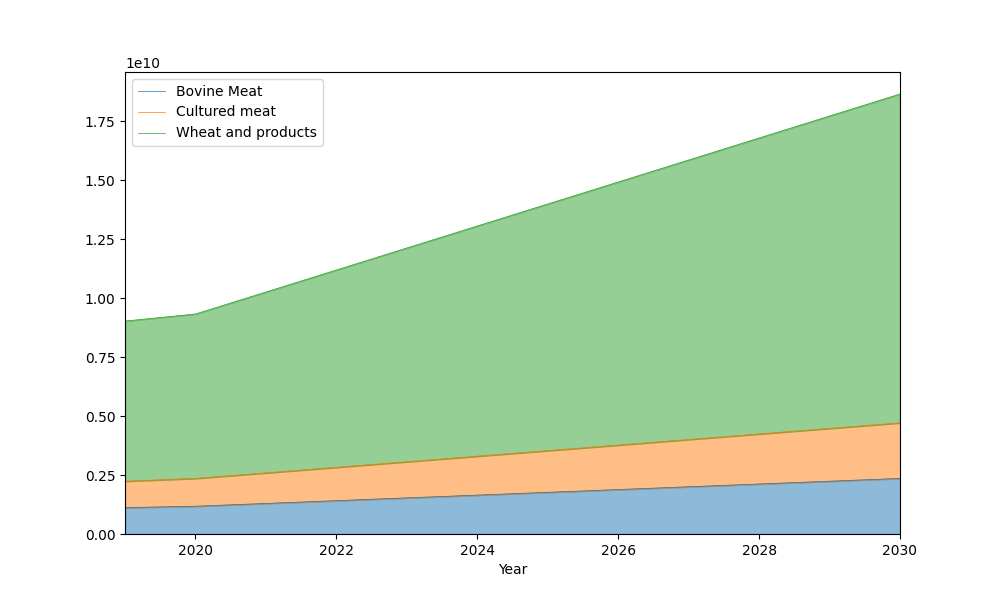
# Get the food results from the pipeline and plot using the fbs accessor
food_results = pipeline.datablock["food"]["food"]

f, ax = plt.subplots(figsize=(10, 6))
food_results.fbs.plot_years(show="Item_name", labels="show", ax=ax)
plt.show()

We can continue adding nodes to the pipeline, even after being executed once. To pick up where we left, we indicate which node to start execution from

# Define a year dependent linear scale starting decreasing at 2021 from 1 to
# 0.5
scaling = linear_scale(
    2019,
    2021,
    2030,
    2030,
    1,
    0.5
)

# We will add a node to scale consumption
pipeline.add_node(
    model.balanced_scaling,
    name="Balanced scaling of items",
    params={
        "fbs": "food",
        "scale": scaling,
        "element": "food",
        "items": ("Item_name", "Bovine Meat"),
        "constant": True,
        "out_key": "food_scaled"
    }
)

# Execute the recently added node
pipeline.run(from_node=8, timing=True)

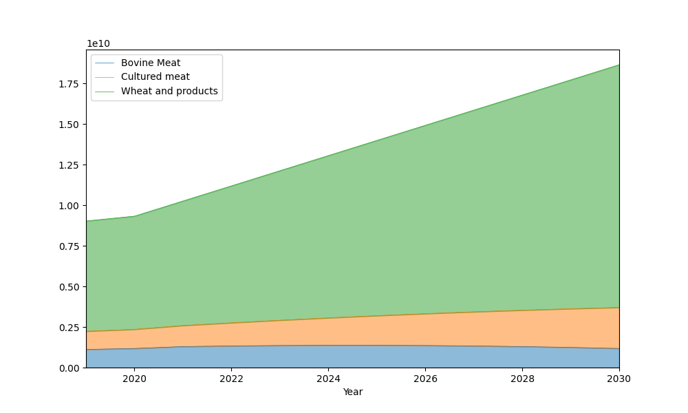
# Get the food results from the pipeline and plot using the fbs accessor
scaled_food_results = pipeline.datablock["food_scaled"]["food"]

f, ax = plt.subplots(figsize=(10, 6))
scaled_food_results.fbs.plot_years(show="Item_name", labels="show", ax=ax)
plt.show()

Node 9: Balanced scaling of items,                       executed in 0.0101 seconds.
Pipeline executed in 0.0102 seconds.

We can see in the scaled Food Balance Sheet that Bovine Meat consumption is reduced by half by 2030, while the total sum across all items remains constant.